11.1 第一个泛函: lapply()
该函数接收函数,以列表形式返回结果。该函数在Base R中是以c语言实现的,所以速度很快。
为了理解该函数的工作机制,考虑一个简单R版本
lapply2 <-  function(x, f, ...) {
  out <- vector("list", length(x))
  #seq_along函数自动获得参数的长度,生成自1开始的序列
  for (i in seq_along(x)) {
    out[[i]] <-  f(x[[i]])
  }
}实际上该函数就对for循环模式的包装器。lapply的优点是减少与循环相关的引用代码,可以更加容易的处理列表。把注意力放在处理函数上。
数据框也是列表,因此可以利用lapply对数据框的列进行操作。
# 获得每一列的类型
unlist(lapply(mtcars, class))
## mpg cyl disp hp drat wt qsec vs
## "numeric" "numeric" "numeric" "numeric" "numeric" "numeric" "numeric" "numeric"
## am gear carb
## "numeric" "numeric" "numeric"# 对每一列求和
unlist(lapply(mtcars, sum))## mpg cyl disp hp drat wt qsec vs
## 642.900 198.000 7383.100 4694.000 115.090 102.952 571.160 14.000
## am gear carb
## 13.000 118.000 90.000lapply有个问题,很难改变调用函数的参数。一种方案就是使用匿名函数。下边例子,将mean函数中的参数trim设置为不同的值。
trims <- c(0, 0.1, 0.2, 0.5)
x <- rcauchy(1000)
unlist(lapply(trims, function(trim) mean(x, trim = trim)))
## [1] 0.64214410 -0.01624563 -0.01692706 -0.0150140611.1.1 循环模式
优先推荐使用这种模式for (i in seq_along(x)),存储和调用效率更高。
三种调用lapply的方式
- lapply(xs function(x) {})
- lapply(seq_along(xs) function(i) {})
- lapply(names(xs) function(nm) {})
通常会使用第一种,可以返回结果。如果需要知道元素的位置,可以考虑第二种和第三种。
11.1.2 练习题
- 下边两种方法,之所以相同,是因为第二种方法,最后一个参数x,传递给mean()函数。
trims <- c(0, 0.1, 0.2, 0.5)
x <- rcauchy(1000)
# \() 替代function(),仅4.1版本支持
lapply(trims, \(trim) mean(x, trim=trim))
## [[1]]
## [1] 1.959715
##
## [[2]]
## [1] 0.08007546
##
## [[3]]
## [1] 0.07435043
##
## [[4]]
## [1] 0.07655139lapply(trims, mean, x=x)## [[1]]
## [1] 1.959715
##
## [[2]]
## [1] 0.08007546
##
## [[3]]
## [1] 0.07435043
##
## [[4]]
## [1] 0.07655139- 对数据框的每一列进行标准化
scale01 <- \(x) {
  rng <- range(x, na.rm = TRUE)
  return((x - rng[1])/(rng[2] - rng[1]))
}
lapply(mtcars, scale01)
## $mpg
## [1] 0.4510638 0.4510638 0.5276596 0.4680851 0.3531915 0.3276596 0.1659574
## [8] 0.5957447 0.5276596 0.3744681 0.3148936 0.2553191 0.2936170 0.2042553
## [15] 0.0000000 0.0000000 0.1829787 0.9361702 0.8510638 1.0000000 0.4723404
## [22] 0.2170213 0.2042553 0.1234043 0.3744681 0.7191489 0.6638298 0.8510638
## [29] 0.2297872 0.3957447 0.1957447 0.4680851
##
## $cyl
## [1] 0.5 0.5 0.0 0.5 1.0 0.5 1.0 0.0 0.0 0.5 0.5 1.0 1.0 1.0 1.0 1.0 1.0 0.0 0.0
## [20] 0.0 0.0 1.0 1.0 1.0 1.0 0.0 0.0 0.0 1.0 0.5 1.0 0.0
##
## $disp
## [1] 0.22175106 0.22175106 0.09204290 0.46620105 0.72062859 0.38388626
## [7] 0.72062859 0.18857570 0.17385882 0.24070841 0.24070841 0.51060115
## [13] 0.51060115 0.51060115 1.00000000 0.97006735 0.92017960 0.01895735
## [19] 0.01147418 0.00000000 0.12222499 0.61586431 0.58094288 0.69568471
## [25] 0.82040409 0.01970566 0.12272387 0.05986530 0.69817910 0.18433525
## [31] 0.57345972 0.12446994
##
## $hp
## [1] 0.20494700 0.20494700 0.14487633 0.20494700 0.43462898 0.18727915
## [7] 0.68197880 0.03533569 0.15194346 0.25088339 0.25088339 0.45229682
## [13] 0.45229682 0.45229682 0.54063604 0.57597173 0.62897527 0.04946996
## [19] 0.00000000 0.04593640 0.15901060 0.34628975 0.34628975 0.68197880
## [25] 0.43462898 0.04946996 0.13780919 0.21554770 0.74911661 0.43462898
## [31] 1.00000000 0.20141343
##
## $drat
## [1] 0.52534562 0.52534562 0.50230415 0.14746544 0.17972350 0.00000000
## [7] 0.20737327 0.42857143 0.53456221 0.53456221 0.53456221 0.14285714
## [13] 0.14285714 0.14285714 0.07834101 0.11059908 0.21658986 0.60829493
## [19] 1.00000000 0.67281106 0.43317972 0.00000000 0.17972350 0.44700461
## [25] 0.14746544 0.60829493 0.76958525 0.46543779 0.67281106 0.39631336
## [31] 0.35944700 0.62211982
##
## $wt
## [1] 0.28304781 0.34824853 0.20634109 0.43518282 0.49271286 0.49782664
## [7] 0.52595244 0.42879059 0.41856303 0.49271286 0.49271286 0.65379698
## [13] 0.56686269 0.57964715 0.95551010 1.00000000 0.97980056 0.17565840
## [19] 0.02608029 0.08233188 0.24341601 0.51316799 0.49143442 0.59498849
## [25] 0.59626694 0.10790079 0.16031705 0.00000000 0.42367681 0.32140118
## [31] 0.52595244 0.32395807
##
## $qsec
## [1] 0.23333333 0.30000000 0.48928571 0.58809524 0.30000000 0.68095238
## [7] 0.15952381 0.65476190 1.00000000 0.45238095 0.52380952 0.34523810
## [13] 0.36904762 0.41666667 0.41428571 0.39523810 0.34761905 0.59166667
## [19] 0.47857143 0.64285714 0.65595238 0.28214286 0.33333333 0.10833333
## [25] 0.30357143 0.52380952 0.26190476 0.28571429 0.00000000 0.11904762
## [31] 0.01190476 0.48809524
##
## $vs
## [1] 0 0 1 1 0 1 0 1 1 1 1 0 0 0 0 0 0 1 1 1 1 0 0 0 0 1 0 1 0 0 0 1
##
## $am
## [1] 1 1 1 0 0 0 0 0 0 0 0 0 0 0 0 0 0 1 1 1 0 0 0 0 0 1 1 1 1 1 1 1
##
## $gear
## [1] 0.5 0.5 0.5 0.0 0.0 0.0 0.0 0.5 0.5 0.5 0.5 0.0 0.0 0.0 0.0 0.0 0.0 0.5 0.5
## [20] 0.5 0.0 0.0 0.0 0.0 0.0 0.5 1.0 1.0 1.0 1.0 1.0 0.5
##
## $carb
## [1] 0.4285714 0.4285714 0.0000000 0.0000000 0.1428571 0.0000000 0.4285714
## [8] 0.1428571 0.1428571 0.4285714 0.4285714 0.2857143 0.2857143 0.2857143
## [15] 0.4285714 0.4285714 0.4285714 0.0000000 0.1428571 0.0000000 0.0000000
## [22] 0.1428571 0.1428571 0.4285714 0.1428571 0.0000000 0.1428571 0.1428571
## [29] 0.4285714 0.7142857 1.0000000 0.1428571- 实现多个公式的线性拟合, data = matcars参数传递给lm()。
formulas <-
  list(mpg ~ disp, mpg ~ I(1 / disp),
       mpg ~ disp + wt,
       mpg ~ I(1 / disp) + wt)
lapply(formulas, lm, data = mtcars)
## [[1]]
##
## Call:
## FUN(formula = X[[i]], data = ..1)
##
## Coefficients:
## (Intercept) disp
## 29.59985 -0.04122
##
##
## [[2]]
##
## Call:
## FUN(formula = X[[i]], data = ..1)
##
## Coefficients:
## (Intercept) I(1/disp)
## 10.75 1557.67
##
##
## [[3]]
##
## Call:
## FUN(formula = X[[i]], data = ..1)
##
## Coefficients:
## (Intercept) disp wt
## 34.96055 -0.01772 -3.35083
##
##
## [[4]]
##
## Call:
## FUN(formula = X[[i]], data = ..1)
##
## Coefficients:
## (Intercept) I(1/disp) wt
## 19.024 1142.560 -1.798- 针对每个bootstraps数据集,进行回归分析
#利用lapply生成数据集,以后应该善用该函数
bootstraps <- lapply(1:10, function(i) {
  # 有放回的重复抽样,因此会有重复记录
  rows <- sample(1:nrow(mtcars), replace = TRUE)
  mtcars[rows, ]
})

# 对10个数据集,分别进行回归分析
lapply(bootstraps, lm, formula = mpg ~ disp)
## [[1]]
##
## Call:
## FUN(formula = ..1, data = X[[i]])
##
## Coefficients:
## (Intercept) disp
## 29.72365 -0.03908
##
##
## [[2]]
##
## Call:
## FUN(formula = ..1, data = X[[i]])
##
## Coefficients:
## (Intercept) disp
## 30.50198 -0.04145
##
##
## [[3]]
##
## Call:
## FUN(formula = ..1, data = X[[i]])
##
## Coefficients:
## (Intercept) disp
## 29.04811 -0.04217
##
##
## [[4]]
##
## Call:
## FUN(formula = ..1, data = X[[i]])
##
## Coefficients:
## (Intercept) disp
## 30.37472 -0.04228
##
##
## [[5]]
##
## Call:
## FUN(formula = ..1, data = X[[i]])
##
## Coefficients:
## (Intercept) disp
## 29.69695 -0.04345
##
##
## [[6]]
##
## Call:
## FUN(formula = ..1, data = X[[i]])
##
## Coefficients:
## (Intercept) disp
## 29.66004 -0.04018
##
##
## [[7]]
##
## Call:
## FUN(formula = ..1, data = X[[i]])
##
## Coefficients:
## (Intercept) disp
## 30.67239 -0.04487
##
##
## [[8]]
##
## Call:
## FUN(formula = ..1, data = X[[i]])
##
## Coefficients:
## (Intercept) disp
## 31.93591 -0.04717
##
##
## [[9]]
##
## Call:
## FUN(formula = ..1, data = X[[i]])
##
## Coefficients:
## (Intercept) disp
## 29.67241 -0.04572
##
##
## [[10]]
##
## Call:
## FUN(formula = ..1, data = X[[i]])
##
## Coefficients:
## (Intercept) disp
## 26.96828 -0.03524- 提取每个模型的\(R^{2}\)
rsq <- \(mod) summary(mod)$r.squared
bootstraps_lm <- lapply(bootstraps, lm, formula = mpg ~ disp)
lapply(bootstraps_lm, rsq)
## [[1]]
## [1] 0.6640258
##
## [[2]]
## [1] 0.7159654
##
## [[3]]
## [1] 0.7656938
##
## [[4]]
## [1] 0.6847409
##
## [[5]]
## [1] 0.7796471
##
## [[6]]
## [1] 0.7198303
##
## [[7]]
## [1] 0.7397383
##
## [[8]]
## [1] 0.7727699
##
## [[9]]
## [1] 0.7726886
##
## [[10]]
## [1] 0.734557911.2 跟lapply相似的泛函数
11.2.1 sapply和vapply
没想到lapply竟然这么有用,可以省略掉非常多的循环。
lapply输出的结果是列表。sapply会自动猜测返回值的类型(列表或向量两种类型)。vapply输出的只是向量类型,但是需要通过FUN.VALUE参数指明返回值的类型。
对于数据框,两个函数返回的都是向量。
sapply(mtcars, is.numeric)## mpg cyl disp hp drat wt qsec vs am gear carb
## TRUE TRUE TRUE TRUE TRUE TRUE TRUE TRUE TRUE TRUE TRUEvapply(mtcars, is.numeric, FUN.VALUE = logical(1))## mpg cyl disp hp drat wt qsec vs am gear carb
## TRUE TRUE TRUE TRUE TRUE TRUE TRUE TRUE TRUE TRUE TRUE针对列表,sapply返回一个空列表,vapply返回一个长度为0的逻辑向量。sapply可能会返回列表,而vapply一直会返回向量。
sapply(list(), is.numeric)## list()vapply(list(), is.numeric, logical(1))## logical(0)下边的情形,sapply会返回列表,因为第二列的类型是2种,而vapply会给出错误提示,因为长度不对。
df <- data.frame(x=1:10,y=letters[1:10])
sapply(df, class)
## x y
## "integer" "character"vapply(df, class, FUN.VALUE = character(1))## x y
## "integer" "character"df2 <- data.frame(x=1:10,y=Sys.time() + 1:10)
sapply(df2, class)## $x
## [1] "integer"
##
## $y
## [1] "POSIXct" "POSIXt"vapply(df2, class, FUN.VALUE = character(1))## Error in vapply(df2, class, FUN.VALUE = character(1)): 值的长度必需为1,
## 但FUN(X[[2]])结果的长度却是2作者模拟了sapply和vapply的函数运行机制。
sapply2 <- \(x, f, ...) {
  res <- lapply2(x, f, ...)
  simplify2array(res)
}

# 对于vapply,判定条件,要求长度和类型都要匹配
vapply2 <- \(x, f, f.value, ...) {
  # n×1列矩阵
  out <- matrix(rep(f.value, length(x), nrow=length(x)))
  for(i in seq_along(x)) {
    res <- f(x[[i]], ...)
    stopifnot(
      length(res) == length(f.value),
      typeof(res) == typeof(f.value)
    )
    out[i,] <- res
  }
  out
}
11.2.2 多重输入:map和mapply
lapply只有第一个参数是可变的,用于计算平均值非常简单,因为mean函数也是只有一个输入参数。
但是如果要操作两个输入参数,怎么办?譬如计算加权均值。 用lapply和vapply也可以操作,但是逻辑相对复杂,不够直接明了。
xs <- replicate(5, runif(10), simplify = FALSE)
ws <- replicate(5, rpois(10,5)+1, simplify = FALSE)
unlist(lapply(seq_along(xs), \(i) {
  weighted.mean(xs[[i]],ws[[i]])
}))
## [1] 0.5321421 0.5146764 0.5205060 0.5279400 0.3761463# vapply
vapply(seq_along(xs), \(i) {
weighted.mean(xs[[i]],ws[[i]])
}, FUN.VALUE = numeric(1))## [1] 0.5321421 0.5146764 0.5205060 0.5279400 0.3761463理用Map函数,可以简单明了的实现对两个数据框操作。但是Map为什么首字母要大写啊,看着别扭,不统一。
与lapply相反,Map函数调用的函数在第一个参数位置,后边跟两个输入列表变量。
unlist(Map(weighted.mean,xs,ws))## [1] 0.5321421 0.5146764 0.5205060 0.5279400 0.3761463通过匿名函数,也可以设定调用函数的参数。
unlist(Map(\(x,w) weighted.mean(x,w, na.rm=TRUE), xs, ws))## [1] 0.5321421 0.5146764 0.5205060 0.5279400 0.376146311.2.3 滚动计算
数据平滑不是很理解。编制一个移动平均值计算函数:
rollmean <- \(x, n) {
  out <- rep(NA, length(x))

  #取小值,譬如2.5会取2
  offset <-  trunc(n / 2)
  for(i in (offset + 1):(length(x) - (n - offset +1))) {
    out[i] <- mean(x[(i-offset):(i+offset-1)])
  }
  out
}
x <- seq(1,3,length=1e2)+runif(1e2)
plot(x)
lines(rollmean(x,6), col="blue",lwd=2)
选取一个窗口,在此范围内的n个数字,用于计算均值。
如果想用中位数,而不是平均值进行绘制,只需要将代码中mean函数改为median即可。但是如果我们不像再建立一个新函数,可以考虑建立一个rollapply函数。
rollapply <- \(x, n, f, ...) {
out <- rep(NA, length(x))
#取小值,譬如2.5会取2
offset <- trunc(n / 2)
for(i in (offset + 1):(length(x) - (n - offset +1))) {
out[i] <- f(x[(i-offset):(i+offset-1)], ...)
}
out
}
x <- seq(1,3,length=1e2)+rt(1e2, df=2) / 2
plot(x)
lines(rollapply(x,6,median), col="red",lwd=2)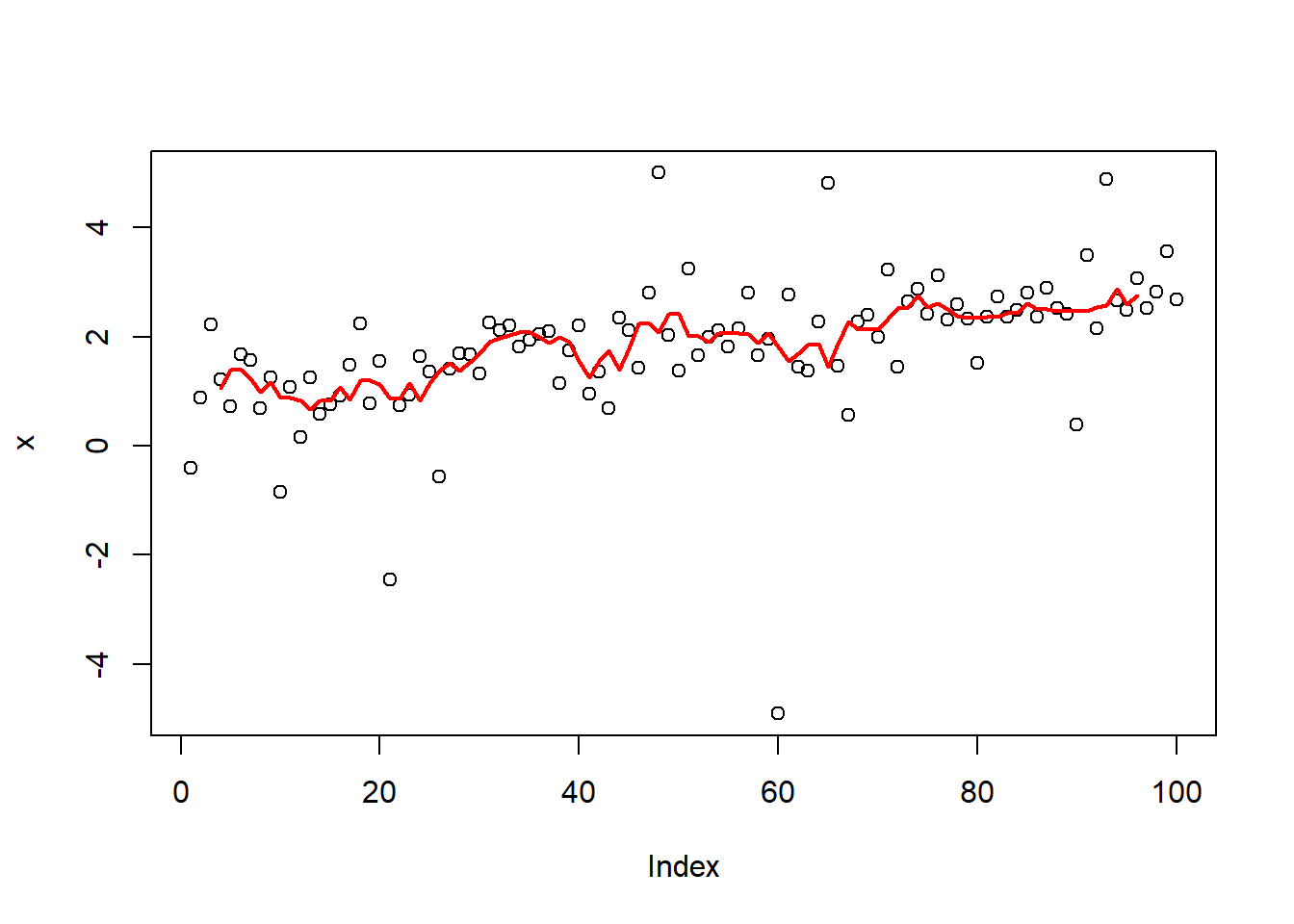 进一步对函数中的循环代码进行改造,试着用vapply代替。
rollapply <- \(x, n, f, ...) {
  #取小值,譬如2.5会取2
  offset <-  trunc(n / 2)
  posis <- (offset + 1):(length(x) - (n - offset +1))
  out <- vapply(posis, \(i) f(x[(i-offset):(i+offset-1)], ...), FUN.VALUE = numeric(1))
  return(out)
}
x <- seq(1,3,length=1e2)+rt(1e2, df=2) / 2
plot(x)
lines(rollapply(x,6,median), col="red",lwd=2)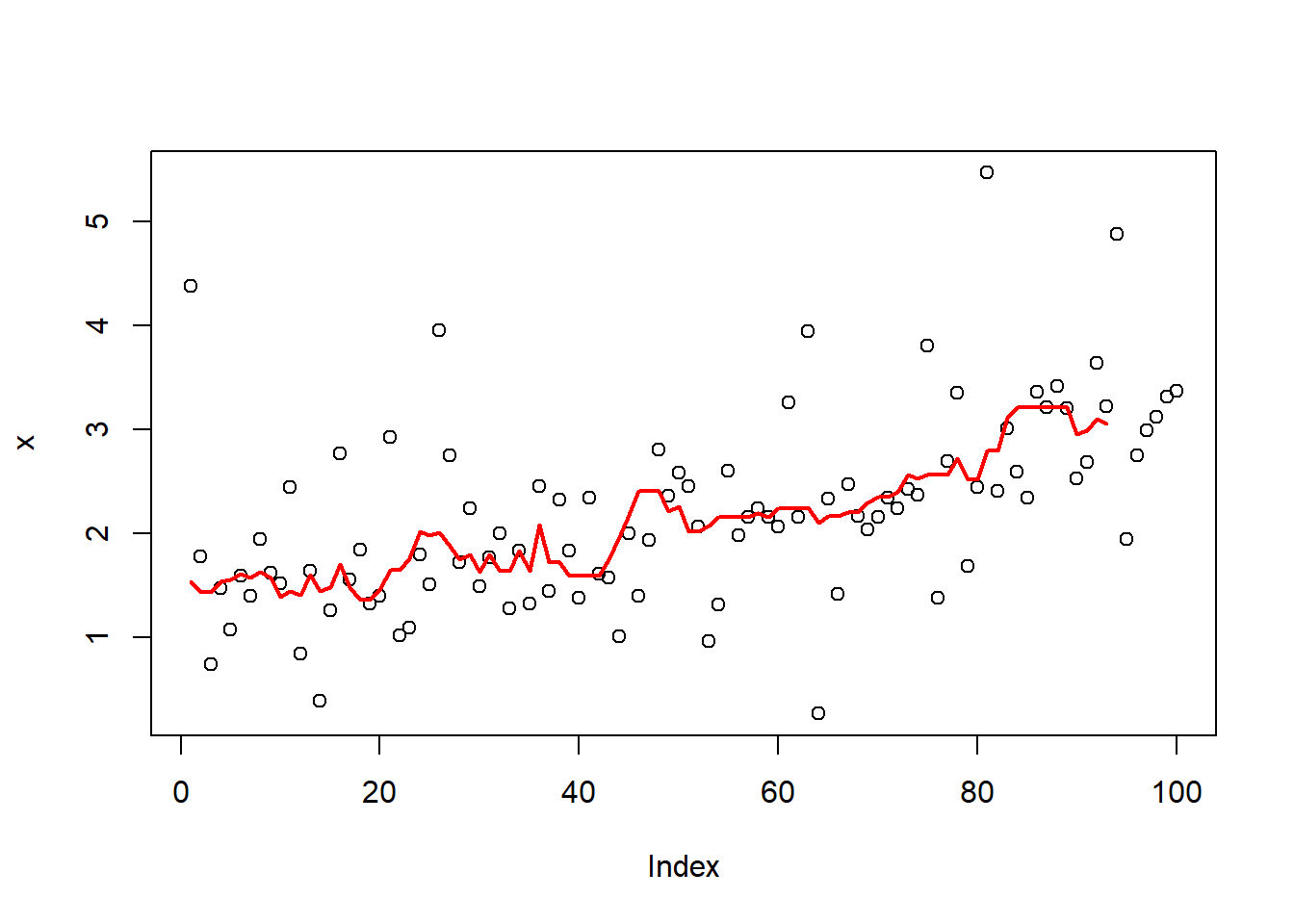
11.2.4 并行
实际上lapply的工作是可以并行的。本文主要是理用parallel包中的几个函数,来提高运算速度。
在windows平台下,貌似不能够真正的进行并行计算,mc.cores参数值只能设置为1。因此下述代码在linux服务器上进行运算。
library(parallel)
boot_df <- function(x) x[sample(nrow(x), replace = TRUE),]
rsquared <- function(mod) summary(mod)$r.square
boot_lm <- function(i) {
  rsquared(lm(mpg ~ wt + disp, data=boot_df(mtcars)))
}

system.time(lapply(1:5000, boot_lm))
system.time(mclapply(1:5000, boot_lm, mc.cores = 4))
并行是有一定的优势:
system.time(lapply(1:5000, boot_lm))
用户 系统 流逝
5.621 0.000 5.620
system.time(mclapply(1:5000, boot_lm, mc.cores = 4))
用户 系统 流逝
4.261 0.396 1.574
但是分派给多个CPU并收集结果,也是需要一些额外的开销,所以看起来mc.cores=8也没有更快。
system.time(lapply(1:5000, boot_lm))
用户 系统 流逝
5.535 0.000 5.534
system.time(mclapply(1:5000, boot_lm, mc.cores = 8))
用户 系统 流逝
4.338 0.566 1.251